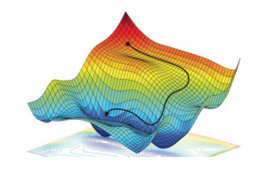
The training (also known as learning or optimisation phase) of neural networks is carried out using the gradient descent method in one of its versions such as back-propagation or stochastic gradient descent. In these methods, the determination of the fit parameters (namely the weights and thresholds of the NN) requires the evaluation of the gradients of ![]() , that is,
, that is,
(1) 
Computing these gradients in the NNPDF case involves handling the non-linear relation between the fitted experimental data and the input PDFs, which proceeds through convolutions both with the DGLAP evolution kernels and the hard-scattering partonic cross-sections as encoded into the optimised APFELgrid fast interpolation strategy.
The theory prediction for a collider cross-section in terms of the NN parameters reads
(2) ![]()
where ![]() indicates a convolution over
indicates a convolution over ![]() ,
, ![]() and
and ![]() stand for the hard-scattering cross-sections and the DGLAP evolution kernels respectively, and sum over repeated flavour indices is understood.
stand for the hard-scattering cross-sections and the DGLAP evolution kernels respectively, and sum over repeated flavour indices is understood.
In the APFELgrid approach, this cross-section can be expressed in a much compact way as
(3) 
where now all perturbative information is pre-computed and stored in the ![]() interpolation tables, and
interpolation tables, and ![]() run over a grid in
run over a grid in ![]() .
.